Part C: Noise, sample size, and comparing systems
The interval on every number
A pass rate from 91 cases is an estimate. If the same system faced 91 different but similar tickets, the rate would come out a bit different. A confidence interval says how different: a 95% interval is a range built so that, over many repetitions, it contains the true rate 95% of the time.
The harness uses the Wilson score interval. For k passes out of n, with z = 1.96 for 95%:
center     = (p + z^2 / 2n) / (1 + z^2 / n)            where p = k / n
half-width = z * sqrt(p(1 - p)/n + z^2 / 4n^2) / (1 + z^2 / n)
Code explained
- In simple words: the formula
wilson()implements, written out so you can check one by hand. - What happens: for the baseline, k = 38 and n = 91, so p = 0.418. The center moves slightly toward 0.5 (0.421), and the half-width is about 0.099, giving 0.322 to 0.520.
- Comes out: the "95% CI 32.2% to 52.0%" in the run summary. Roughly: with 91 cases, any pass rate between 40% and 60% is uncertain by about 10 points either way.
The noise floor
The interval covers sampling of cases. A stochastic system adds a second source of variation: the same cases give different results on each run. The noise floor is how much the score moves when nothing changed. Measure it before you believe any improvement smaller than it.
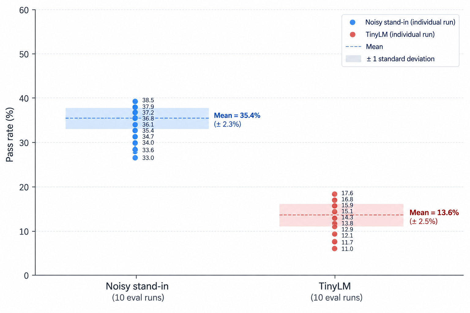
The harness measures it directly: run the system several times with different seeds on the same 91 cases and look at the spread. Two stochastic systems are available here. noisy is the version 1 baseline plus seeded random faults (15% of cases get a wrong category, a dropped citation, an added roadmap promise, or truncated JSON): a simulation that behaves like a flaky model, not a model. tinylm is real: the reply is sampled from TinyLM at temperature 0.7.
python examples/m10_evals.py noise --system noisy --runs 10
python examples/m10_evals.py noise --system tinylm --runs 10
Code explained
- In simple words: run each system ten times without changing anything and see how far the score wanders.
- What happens:
noise_floorcalls the system factory with seeds 0 to 9, runs all 91 cases each time without saving, and records each run's pass rate and each case's pass or fail per run. A case that passed in some runs and failed in others is "flaky". - Comes out: (the TinyLM run takes about 20 seconds on two CPU cores with one thread; the other is instant)
noisy: 10 runs x 91 cases
pass rates: 0.330 0.363 0.341 0.385 0.385 0.363 0.363 0.352 0.352 0.374
mean 0.360  stdev 0.018  range 0.330 to 0.385
cases that flipped at least once: 31 of 91
tinylm: 10 runs x 91 cases
pass rates: 0.121 0.132 0.154 0.176 0.132 0.121 0.154 0.110 0.132 0.154
mean 0.138  stdev 0.020  range 0.110 to 0.176
cases that flipped at least once: 15 of 91

real	0m21.960s
user	0m21.403s
sys	0m0.239s
Both systems move by about 2 points of standard deviation and span 5.5 to 6.6 points between their best and worst run, with no change at all. So a single run of a stochastic system that "improves" by 4 points has told you nothing. TinyLM's rate is low (its replies are mostly memorized fragments), but the lesson is the spread, not the level. The flaky-case list is also useful: those cases are where the system is unsure, and they are good candidates for a closer look.
To measure the floor of a real model, run the same command with --system llm. At temperature 0 hosted models still vary somewhat between calls; at the temperatures you use in production they vary more. Five runs are a reasonable minimum; each costs one full eval.
How many cases do you need?
Statistical power is the chance an experiment detects a difference that really exists. The convention is 80% power at a 5% significance level (a 5% chance of a false alarm). The number of cases you need depends on the size of the difference and on whether the comparison is paired.
For two systems each scored on its own independent cases, the classic formula per system, for rates p1 and p2, is:
n = ( z_a * sqrt(2 * pbar * (1 - pbar)) + z_b * sqrt(p1(1 - p1) + p2(1 - p2)) )^2 / (p1 - p2)^2
z_a = 1.96 (two-sided 5%), z_b = 0.8416 (80% power), pbar = (p1 + p2) / 2
Code explained
- In simple words: the unpaired sample-size formula that
n_two_proportions()implements. - What happens: for 80% vs 85%: pbar = 0.825, the first term is 1.96 x 0.5373 = 1.0532, the second is 0.8416 x 0.5362 = 0.4513, their sum squared is 2.2634, and dividing by 0.05 squared gives 905.4, rounded up to 906 per system.
- Comes out: 906 cases per system to detect a 5-point difference reliably. A 91-case eval is about a tenth of that.
Pairing helps a lot. When both systems run on the same cases, cases that both pass or both fail carry no information about the difference; only discordant cases (one passes, the other fails) do. The paired sample size depends on how often the systems disagree:
n = ( z_a * sqrt(d_rate) + z_b * sqrt(d_rate - delta^2) )^2 / delta^2
d_rate = share of cases only B passes + share only A passes;  delta = their difference
Code explained
- In simple words: the paired (McNemar) sample-size formula that
n_mcnemar()implements. - What happens: if B alone passes 7.5% of cases and A alone passes 2.5% (a 5-point net gain with 10% disagreement): 1.96 x sqrt(0.1) = 0.6198, 0.8416 x sqrt(0.0975) = 0.2628, the sum squared is 0.7790, divided by 0.0025 gives 311.6, so 312 cases.
- Comes out: 312 paired cases instead of 906 per arm, because pairing removes the variation from case difficulty.
The script prints the whole picture:
"""Module 10, Part C: how many eval cases do you need?

    PYTHONPATH=. python examples/m10_power.py
"""
from __future__ import annotations

from examples.m10_stats import n_mcnemar, n_two_proportions, wilson

print("Unpaired: two systems, each on its OWN random cases (alpha 0.05, power 0.8)")
for p1 in (0.60, 0.80, 0.90):
    print(f"  {p1:.0%} vs {p1 + 0.05:.0%}: {n_two_proportions(p1, p1 + 0.05):>5} cases per system")

print("Paired: both systems on the SAME cases; only cases where they disagree carry information")
for only_b, only_a in ((0.10, 0.05), (0.075, 0.025), (0.05, 0.0)):
    print(f"  B-only {only_b:.1%}, A-only {only_a:.1%} (discordant {only_b + only_a:.1%}): "
          f"{n_mcnemar(only_b, only_a):>5} cases")

print("What n=91 can resolve: 95% Wilson interval half-width at each pass rate")
for p in (0.4, 0.6, 0.8, 0.9):
    lo, hi = wilson(round(p * 91), 91)
    print(f"  {p:.0%}: {lo:.1%} to {hi:.1%}  (about +/- {(hi - lo) / 2 * 100:.1f} points)")

print("Smallest paired improvement detectable with 91 cases, if 1 in 20 cases also gets worse:")
for d in (0.05, 0.08, 0.10, 0.12, 0.15):
    need = n_mcnemar(d + 0.05, 0.05)
    print(f"  +{d:.0%} net: needs {need:>4} cases" + ("  (fits in 91)" if need <= 91 else ""))
Code explained
- In simple words: four small tables computed from the formulas above.
- What happens: it imports
n_two_proportions,n_mcnemar, andwilsonfromm10_stats.pyand loops over a few scenarios; nothing is simulated. - Comes out: see the run below.
python examples/m10_power.py
Code explained
- In simple words: sample sizes for a 5-point difference, and what 91 cases can and cannot tell apart.
- What happens: it prints the unpaired sample size at three baseline rates, the paired sample size at three disagreement levels, the Wilson interval width for 91 cases at several pass rates, and the smallest paired net improvement 91 cases could detect when 5% of cases also get worse.
- Comes out:
Unpaired: two systems, each on its OWN random cases (alpha 0.05, power 0.8)
  60% vs 65%:  1471 cases per system
  80% vs 85%:   906 cases per system
  90% vs 95%:   435 cases per system
Paired: both systems on the SAME cases; only cases where they disagree carry information
  B-only 10.0%, A-only 5.0% (discordant 15.0%):   469 cases
  B-only 7.5%, A-only 2.5% (discordant 10.0%):   312 cases
  B-only 5.0%, A-only 0.0% (discordant 5.0%):   155 cases
What n=91 can resolve: 95% Wilson interval half-width at each pass rate
  40%: 30.1% to 49.8%  (about +/- 9.9 points)
  60%: 50.2% to 69.9%  (about +/- 9.9 points)
  80%: 70.9% to 87.1%  (about +/- 8.1 points)
  90%: 82.3% to 94.7%  (about +/- 6.2 points)
Smallest paired improvement detectable with 91 cases, if 1 in 20 cases also gets worse:
  +5% net: needs  469 cases
  +8% net: needs  219 cases
  +10% net: needs  155 cases
  +12% net: needs  118 cases
  +15% net: needs   85 cases  (fits in 91)
The practical reading for Brightlane: 91 cases resolve a pass rate to about plus or minus 10 points, and reliably detect only a net improvement of about 15 points. To detect 5-point differences you need 300 to 500 paired cases, which is the target for the golden set as production traffic arrives (Part G). Until then, say "not yet shown" about small gains, not "better".
| Situation | Use this | Why |
|---|---|---|
| Two versions on the same cases (the normal eval) | Paired test: exact McNemar for "is there a difference", paired bootstrap for "how big" | Needs far fewer cases than an unpaired test |
| Two groups of different users (an A/B test) | Two-proportion z test, sample size from n_two_proportions | Users are not paired; each sees one version |
| One stochastic system, is a change real? | Measure the noise floor first; compare means over several runs | A single run's gain can be pure noise |
| Very few discordant cases (under about 25) | Exact McNemar, not the chi-squared approximation | The approximation is poor for small counts |
Error analysis before optimization
Before changing anything, find out why cases fail. Error analysis means reading failed cases and tagging each with a cause from a small taxonomy (a fixed list of failure types), then counting. It turns "the pass rate is 42%" into "fix these two things first".
The taxonomy in failure_tags is ordered upstream first: broken output, then retrieval misses, wrong reply language, wrong category, missed escalation, ungrounded reply, and policy violation. Each cause splits by language when language matters, because "retrieval missed a Spanish ticket" and "retrieval missed an English ticket" need different fixes. A sole cause is a case's only problem: fixing it alone turns that case green, which makes sole-cause counts the best estimate of what a fix is worth.
Do this on the dev split only. The test split stays untouched until the end, so it can tell you whether your fixes generalize.
python examples/m10_evals.py errors runs/baseline.json --tag dev --show wrong_category,missed_escalation,policy_violation
Code explained
- In simple words: count failure causes on the 48 dev tickets and print the cases behind three of them.
- What happens:
error_analysistags each failed dev case, counts all causes and sole causes, and--showprints each matching case with the details of its failed checks. - Comes out:
Notice what the analysis says not to do yet. Non-English failures (6 wrong language, 6 wrong category, 5 retrieval misses) are large, but no case has them as a sole cause: every non-English case fails three ways at once, so fixing one of the three moves nothing. That needs a different system (a real model, or translation before retrieval), not a keyword tweak.
After the fix, the regression cases go in:
python examples/m10_evals.py run --system baseline_v2
python examples/m10_evals.py regress T-1028 T-1029 T-1058 --reason "v1 copied a roadmap quarter from the KB; fixed in v2"
Code explained
- In simple words: score the fixed version, then lock the three roadmap cases into the regression suite.
- What happens: the run writes
runs/baseline_v2.json.regresscopies the three golden records intoevals/regressions.jsonlwith the reason and date. - Comes out:
Is v2 really better? Paired comparison
Two intervals (32% to 52%, and 50% to 70%) barely overlap, which tempts people to say "not significant". That reasoning is wrong for paired data: both systems ran on the same cases, so compare case by case.
bashCopy
python examples/m10_evals.py compare runs/baseline.json runs/baseline_v2.json
Code explained
- In simple words: line the two runs up case by case and count where they disagree.
- What happens:
comparechecks both runs used the same golden fingerprint, lists cases only one system passes, computes the exact McNemar p-value and the paired bootstrap interval, and repeats the discordant count and McNemar test within each split. - Comes out:
baseline 41.8%  vs  baseline_v2 60.4%  on n=91 paired cases
only baseline passes: 0 []
only baseline_v2 passes: 17 ['H-15', 'H-17', 'H-18', 'H-19', 'T-1016', 'T-1025', 'T-1028', 'T-1029', 'T-1039', 'T-1040', 'T-1049', 'T-1050', 'T-1055', 'T-1058', 'T-1063', 'T-1068', 'T-1070']
difference +0.187 (paired bootstrap 95% CI +0.110 to +0.275)  McNemar exact p=0.0000
  dev      baseline  22/48   baseline_v2  33/48   discordant 0/11  McNemar p=0.001
  test     baseline  11/24   baseline_v2  13/24   discordant 0/2  McNemar p=0.500
  curated  baseline   5/19   baseline_v2   9/19   discordant 0/4  McNemar p=0.125
Overall the result is clear: 17 cases improved and none got worse. Under "no difference", 17 of 17 discordant cases going one way has probability 2 x 0.5^17, about 0.000015, and the bootstrap puts the gain at 11 to 27.5 points. Now look at the splits. On dev, where the fixes were designed, 11 of 11 discordant cases improved. On the held-out test split only 2 cases changed (p = 0.5): the data cannot tell a real gain there from luck. That is the honest summary: v2 is better on the cases we studied; on unseen tickets the improvement is not yet shown. Rules written by reading dev failures fit dev failures. This is the same overfitting Module 4 warned about with prompts, and the reason the test split exists.